
読み込み中...
読み込み中...
Cabernet2D is a two-dimensional flow and riverbed evolution solver introduced in iRIC V4. Based on Nays2dH and Nays2dFlood, it combines river confluences and bifurcations, levee breach simulations, a riverine tree lifecycle model, and structures such as culverts and groynes in a single solver. Its unstructured grid also supports the modeling of complex river networks.
For detailed instructions, see the Cabernet2D Manual.
The following features were added on July 3, 2026:
Parallel computation using OpenMP.
An option to account for energy losses in flow over a downward bed step.
An avalanche treatment for steep slopes at a delta front.
Full support for riverbed evolution with mixed-size bed load and suspended load.
Improved sediment mass conservation for mixed grain sizes, particularly in suspended-load calculations.
Upstream sediment supply conditions for suspended load and bed load that can be adjusted using multipliers relative to equilibrium conditions.
Three quasi-three-dimensional flow methods: (0) Engelund's equilibrium secondary flow, (1) the Nays2dH transport equation for secondary-flow intensity, and (2) the Uchida–Fukuoka BVC (Bottom Velocity Computation) method with dispersion terms and dynamic pressure correction (updated on October 7, 2026; see below).
Features added on July 31, 2026
An option to include or exclude dispersion terms arising from the difference between the vertical velocity distribution and the depth-averaged velocity in the BVC method.
New boundary conditions, "Inflow from an upper floor" and "Outflow to a lower floor," for simulations of flooding on the ground surface and in underground spaces with multiple levels.
Features added on August 3, 2026
The discharge formula for outflow to underground spaces ("Outflow to a lower floor": UndergroundExit) was changed to the empirical equation Q=c1·B·H^c2 from the Japanese Ministry of Land, Infrastructure, Transport and Tourism's guidelines for flood protection in underground spaces. Here, B is the entrance width and H is the surface inundation depth; the default coefficients are c1=1.59 and c2=1.65.
Both "Inflow from an upper floor" (UndergroundEntrance) and "Outflow to a lower floor" (UndergroundExit) now allow one of four flow directions (±i or ±j) to be specified. Faces other than those in the specified direction are automatically made impermeable.
Surface flood simulations can now account for the building coverage ratio and building resistance, following Section II.4 of the Nays2dFlood Solver Manual. When the grid is too coarse to represent individual buildings, reduced cell porosity and effective flow area at cell faces, together with building drag, provide a simplified representation of flow concentrating along roads beside buildings.
Features added on October 7, 2026
Features added on October 22, 2026
Elevation_fix) issue was corrected. During avalanche treatment or riverbed evolution calculations involving suspended load (bed-load/suspended-load formula selection ≥2), erosion could previously extend below the specified fixed-bed depth.Features added on November 5, 2026
Downstream boundaries in complex river networks now support Manning normal-depth conditions based on each outlet's own discharge. An initialization omission that could cause calculations to diverge was also corrected. This improves stability at bifurcations where the main channel and branches have independent receiving-water levels.
An instability in streamline-curvature calculations in cells adjacent to obstacles such as partition walls was corrected. Calibration coefficients for secondary-flow intensity and vorticity were also added.
Simulate confluences and bifurcations without a limit on the number of tributaries or branches. Discharge or water-level boundary conditions can be specified at every upstream inlet, and water-level boundary conditions at every downstream branch outlet.
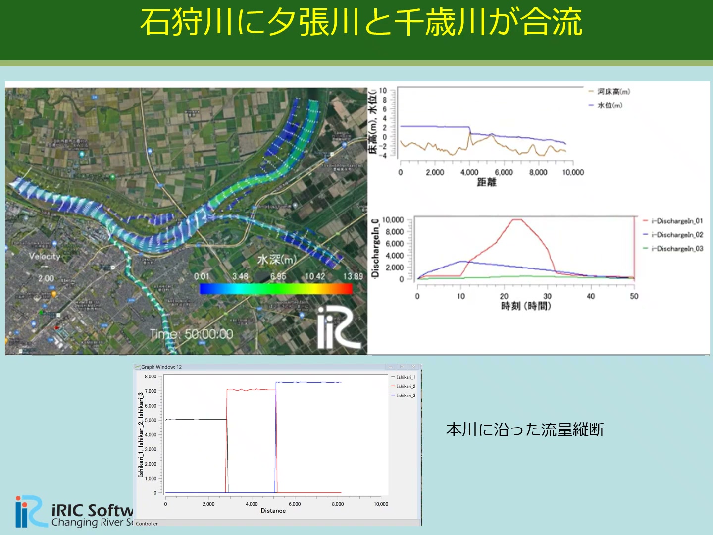 Velocity distribution, longitudinal water-surface and bed profiles, and discharge hydrographs at the confluence of the Chikugo and Katsura rivers. Data courtesy of Yasuda, Shirakawa, and Kamoshida (2025).
An unstructured grid enables integrated simulations of complex river networks with multiple confluences and bifurcations. Discharge and sediment transport through arbitrary cross sections can also be displayed. General-purpose grid-generation tools simplify mesh creation.
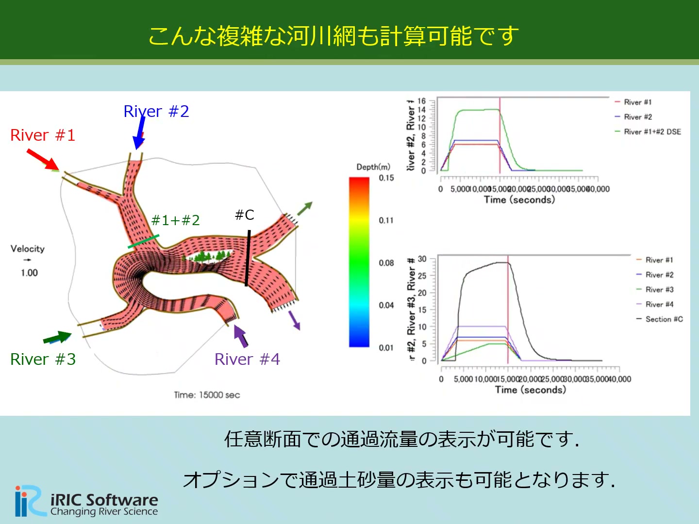 Example of a network in which four rivers (River #1–#4) merge and divide, showing discharge through arbitrary cross sections.
Introductory Video
iRIC V4 New Solver: Cabernet2D (YouTube)Trial Version
Trial versions of Cabernet2D and Freebird 3D are available for everyone. Please feel free to contact us for installation guidance, usage instructions, short workshops, demo presentations, or any other inquiries.
Full Version (Gold Members Only)
The full version is available as a benefit for iRIC-UC Gold Members. An online workshop (approximately half a day) is also included in the Gold Member benefits.
Simulate sediment deposition and riverbed evolution at confluences. A tree lifecycle model—germination, growth, flow resistance, and washout—is integrated into the riverbed evolution loop, allowing long-term processes such as bar formation, tree establishment, woodland development, and bar stabilization to be reproduced.
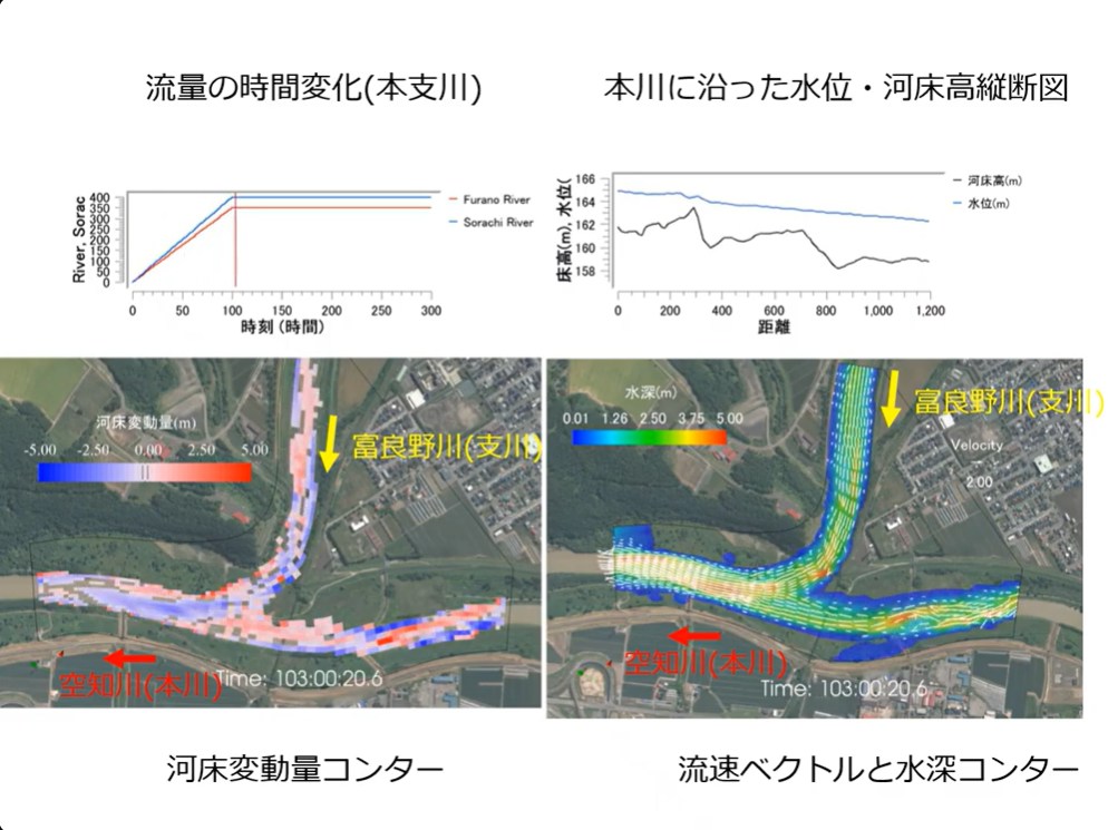
Riverbed elevation change contours and velocity vectors at the confluence of the Sorachi River (main channel) and the Furano River (tributary). |
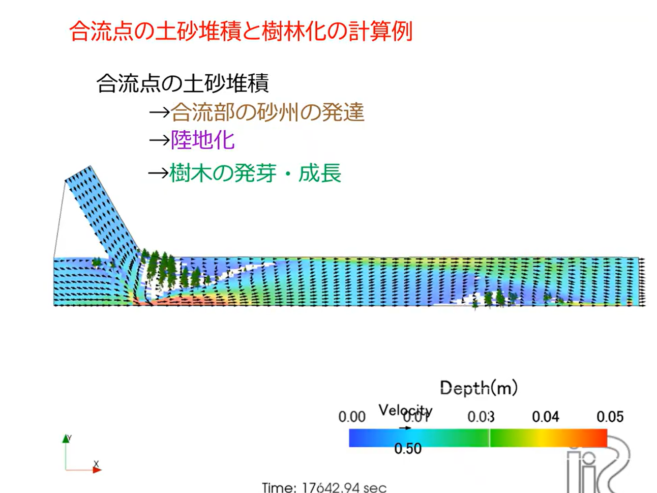
Sediment deposition at a confluence, followed by bar development, emergence above water, and tree germination and growth. |
Simulate bifurcations that conventional Nays2DH could not handle. Both the main channel and branches can start from dry conditions, with discharge partitioning determined automatically by the model. Simulations with riverbed evolution can reproduce a decrease in branch discharge as sediment accumulates in the branch. Each branch outlet can use its own Manning normal-depth boundary condition based on its discharge, supporting natural bifurcations with independent receiving-water levels, such as delta distributaries flowing separately into the sea.
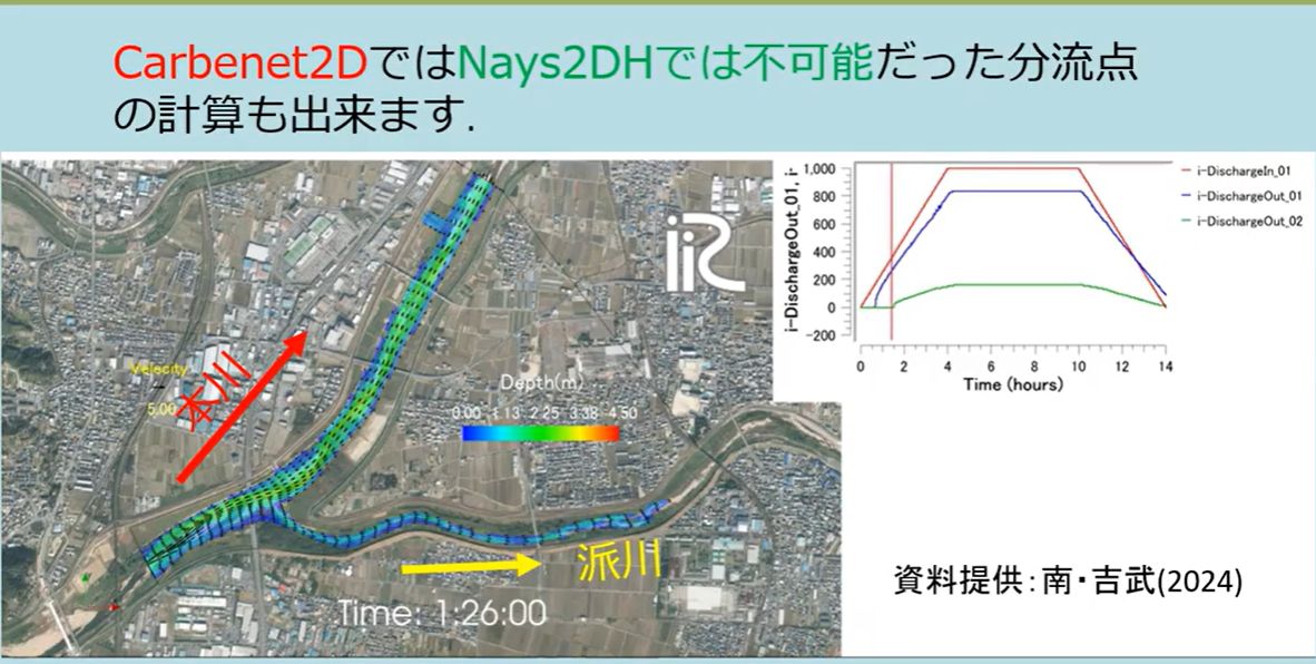 Example starting with dry conditions in both the main channel and the branch, with discharge partitioning determined automatically. Materials courtesy of Minami and Yoshitake (2024).
Simulate levee breaches with coordinated views of three-dimensional bed and water-surface topography and plan-view flow fields. Accuracy has been assessed through comparisons with experimental results.
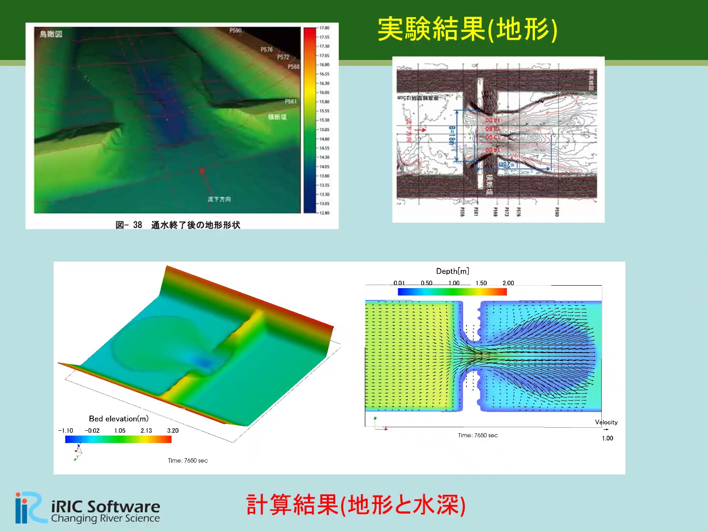 Reproduction of a large-scale levee breach experiment at the Chiyoda Experimental Channel. Top: experimental topography. Bottom: simulated topography and water depth. Experimental data: Shimada et al., Civil Engineering Research Institute for Cold Region (2012).
Define obstacles along grid edges to represent very thin permeable or impermeable groynes. Permeability and vorticity can be displayed. Simulations can also represent the control of alternate bars by groynes, sediment deposition between groynes, and tree establishment.
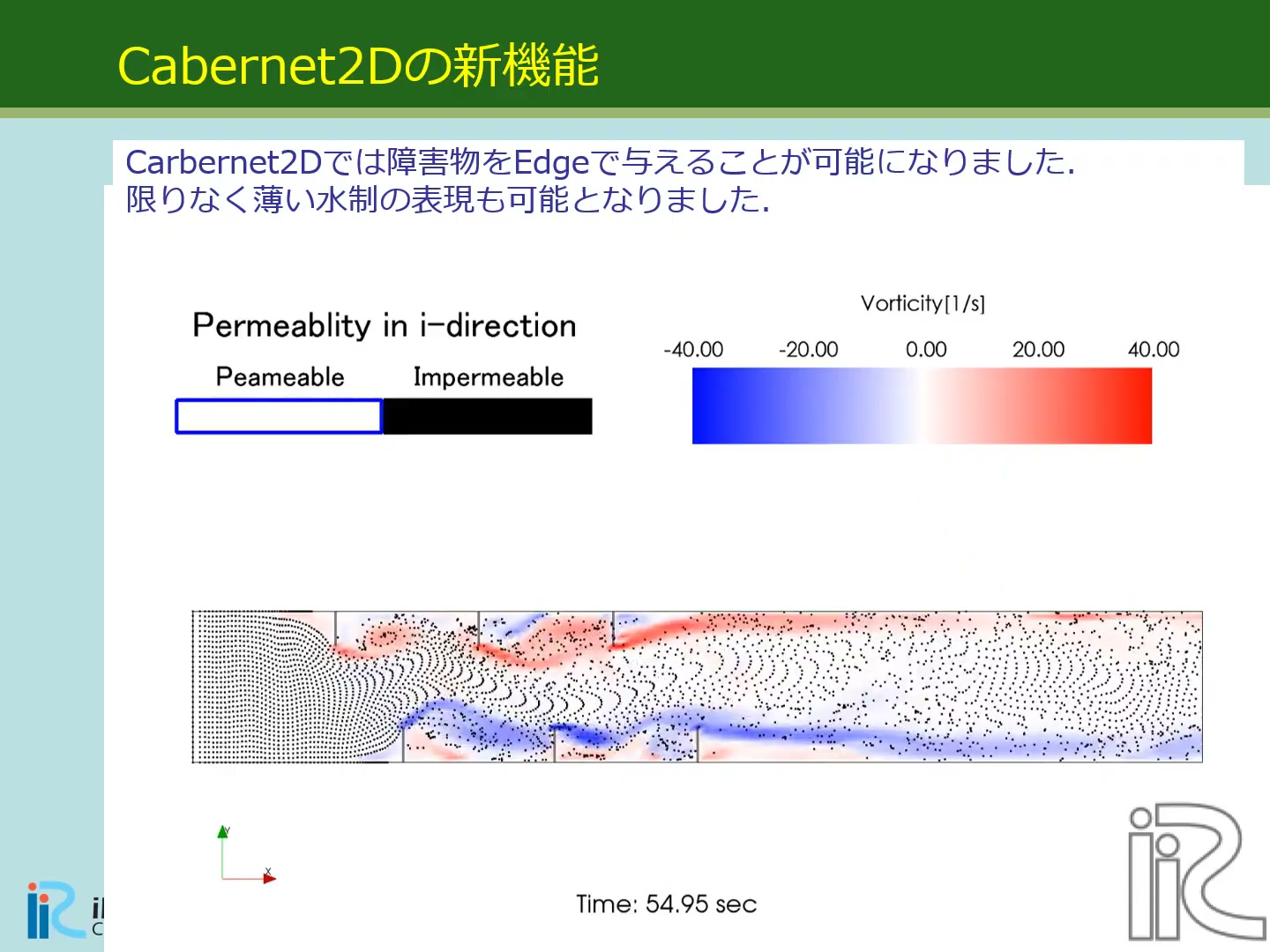 Velocity vectors around groynes represented by edge obstacles, with permeability and vorticity distributions.
The built-in GELATO model places neutrally buoyant particles in the near-bed and surface flows to simulate transport using a Lagrangian approach. It can be used to visualize flow.
Upstream and downstream boundary conditions based on Riemann invariants provide a more accurate alternative to Manning-based conditions. Validation against a 1:50-scale physical model of the upper Ishikari River showed close agreement between simulated and experimental discharge.
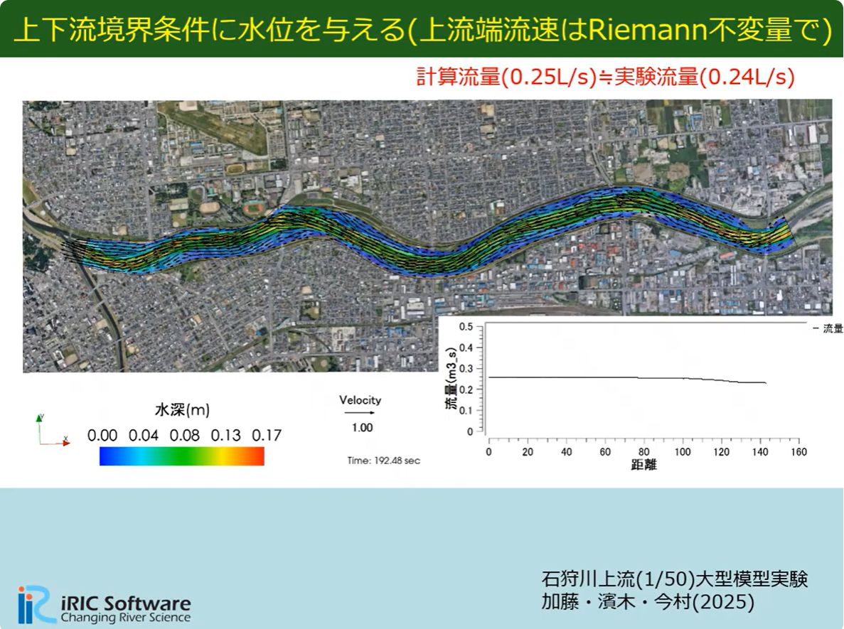 Boundary conditions using Riemann invariants: simulated discharge (0.25 L/s) ≈ experimental discharge (0.24 L/s). Kato, Shimizu, and Imamura (2025).
Simulate flow around floodplain structures including culverts, sluice gates, drainage outlets, drainage pumps, and gates.
Link surface flood simulations with flooding in underground spaces such as shopping areas and subway stations. Assigning the "Outflow to a lower floor" boundary condition to surface cells representing stairway or escalator entrances automatically outputs an inflow time series (CSV) based on surface inundation depth and the empirical equation Q=c1·B·H^c2 from the Japanese Ministry of Land, Infrastructure, Transport and Tourism's guidelines. This CSV can then be used as the discharge input for the "Inflow from an upper floor" boundary condition in a separate underground model, enabling linked surface–underground flood simulations. Both boundary conditions support four flow directions (±i or ±j), with faces outside the specified direction automatically made impermeable.
When an urban flood grid is too coarse to resolve individual buildings, a building coverage ratio can be assigned to each cell to approximate how building groups concentrate and divert floodwater, following the Nays2dFlood Solver Manual. Cell porosity and effective flow area at cell faces are reduced according to the coverage ratio, and building drag is added to the momentum equations. Options are available for including or excluding inundation inside buildings and for selecting the face-porosity evaluation method (symmetric arrangement or mosaic arrangement).